Help
1. Set up a search :
2. Watch the progress of the analysis workflow.
3. Explore results.
4. Select hits of interest
5. Export selection
Focus on Genomic Co-location Filtering
1. Set up a search
Go to the application's input tab.
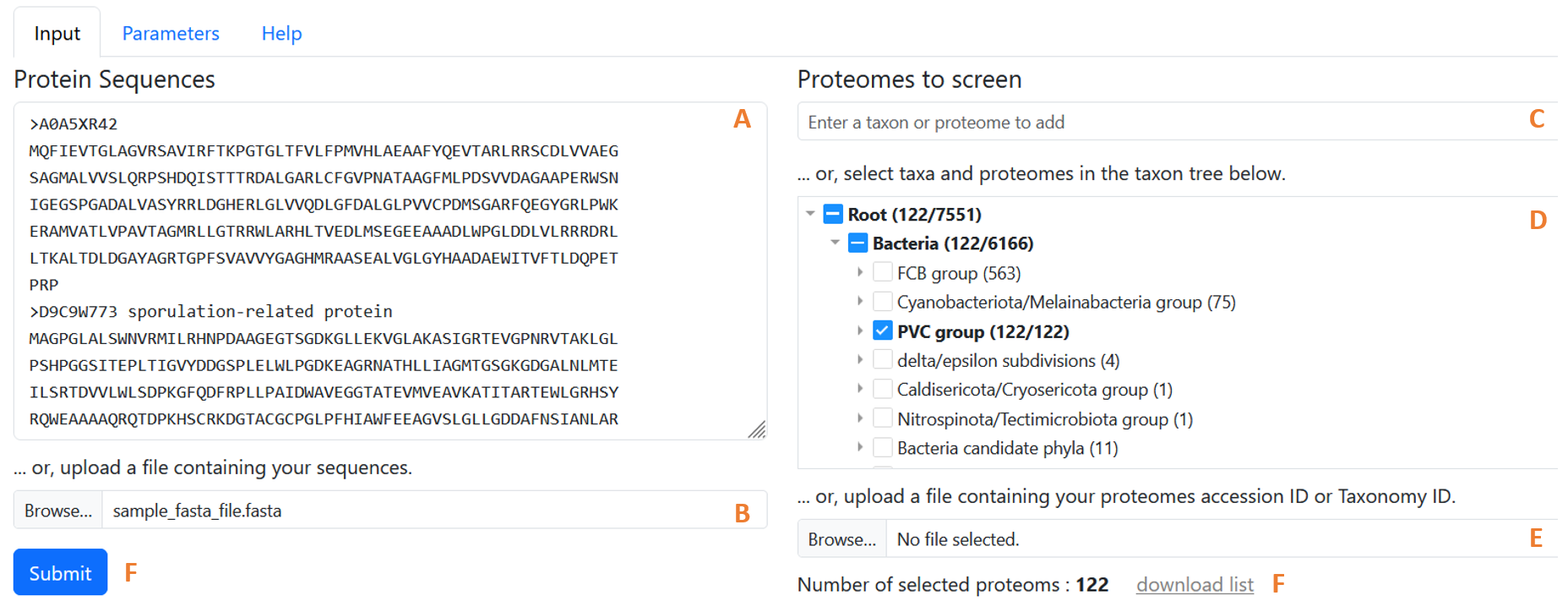 Figure 1: The WHOPPER browser with its key features on raw alignments.
1. Enter proteins to search [required]
Fill in the Protein Sequences field with one or more protein sequences in fasta format. This field can be filled in in one of two ways:
- By manually entering the sequences in the appropriate text field. (figure 1.A)
- By uploading a file containing the protein sequences to be analyzed. (figure 1.B)
Note: The number of sequences that can be analyzed at once is limited. This limit is set by the administrator of the instance you are using.
2. Select the proteomes to screen. [required]
The choice of dataset to screen is made by selecting proteomes of interest individually or by taxa. When a taxon is selected, all proteomes associated with that taxon are selected. The number of proteomes in the current selection is shown at the bottom of the page (figure 1.F). The list of proteomes in the current selection can also be downloaded (figure 1.G).
Three complementary functions can be used to define the reference proteome to be screened:
- The autocompletion list (figure 1.C) allows you to search the list of proteomes and taxa for those you wish to add to the dataset. Entering a few letters will bring up the list of corresponding taxa/proteomes. Each item includes a taxon name and the number of proteomes associated with it. If the taxon itself or a sub-taxon has already been selected, the number of proteomes already selected is also indicated. Clicking on an item in the list allows the corresponding proteomes to be added or removed from the selection. Clicking on an item corresponding to a taxon already selected (even partially) removes all proteomes associated with this taxon from the selection.
- The taxon tree (figure 1.D) lets you browse the tree of available taxa, and directly select taxa/proteomes of interest from this tree. Each node of the tree includes a taxon name and the number of proteomes associated with it. If the taxon itself or a taxon sub-taxon has already been selected, the number of proteomes already selected is also indicated. Clicking on the triangle icon in front of each node allows the sub-taxa to appear or disappear. Clicking on the square icon in front of each node allows the corresponding proteomes to be added or removed from the selection.
- The selection by importing a list from a file (figure 1.E) allows users to utilize a file containing a list of proteome accession numbers or taxon IDs to add the corresponding proteomes or those belonging to the specified taxon IDs to the current selection. The file must contain an accession number, or taxon id on each line of the file in the first column. The file must be in text format (extension .txt or .tsv) and the separators used may be tab, comma or semicolon.
Notes:
- The number of proteomes that can be screened at once is limited. This limit is set by the administrator of the instance you are using. If this limit is exceeded, the number of selected proteomes (figure 1.F) will appear in red.
- It is possible to obtain the complete list of proteomes available in the instance you are using and their corresponding accession numbers. To do this, select all the proteomes available via the autocompletion list or the taxonomic tree, then click on the “download list” link.
3. Modify search parameters [optional]
In the application's a parameters tab, the following search parameters can be modified: some search parameters can be modified:
General settings :
Retrieve hits locations information : activate this option to add the genomic location of hits to the results. This option is required to use the genomic hit colocation filter in the results exploration interface. (see the section Genomic co-location filtering)
Results filtering criteria :
- Maximum number of hits reported : maximum number of HMMER hits reported for each query for each proteome.
- Maximum hit e-Value : maximum e-value allowed for reported HMMER hits.
- Maximum hit Identity : minimum percentage of identity allowed for reported HMMER hits.
- Minimum hit similarity : minimum percentage of similarity allowed for reported HMMER hits.
- Minimum hit length : minimum hit length allowed for reported HMMER hits.
- Minimum hit coverage on queries : minimum percentage of the query sequence that must be covered for reported hits.
Note: All these criteria will be used to pre-filter the alignment results, which can help limit the amount of data handled by the application and thus guarantee its responsiveness. However, it is not recommended to be too stringent at the pre-filtering stage, as these filters (except e-value) can be adjusted directly in the exploration interface according to the results obtained.
4. Submit the form [required]
In the application's input tab, use the “submit” button (Figure 1.G) to launch the search.
Once the search is launched, you'll be redirected to a url associated with your search. This url will allow you to access the results of your search for a certain duration. Depending on your search status, the corresponding tab will be displayed by default. Immediately after launching the search, you'll be directed to the “running” tab (see section “Watch the progress of the analysis workflow”). When the search is complete, you'll be redirected to the “Results” display page (see “Explore results”).
Note : Once the search is launched, you'll have access to the input and parameters tabs of your search. However, you won't be able to configure and relaunch a new search from here. To relaunch a search, you'll need to use the “New search” tab.
2. Watch the progress of the analysis workflow
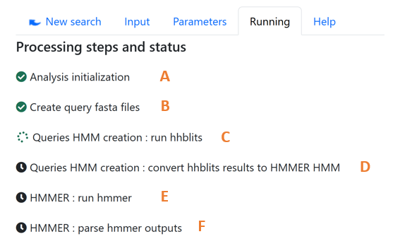 Figure 2: Analysis workflow monitoring showing status of each processing step from initialization to HMMER output parsing.
Once the search is running, you can follow the progress of the analysis workflow via the “Running” tab.Once the search is running, you can follow the progress of the analysis workflow via the “Running” tab. In front of each step, an icon indicates its status: pending, in progress, completed, failed.If a step has failed, the error is displayed below it.
Description of steps
- Analysis initialization (Figure 2.A): The search parameters are recorded, a unique url is assigned to it.
- Create query fasta file (Figure 2.B): A fasta file is created for each sequence provided.
- Queries HMM creation (Figure 2.C): HHblits is used to align each sequence against the Uniref database. These alignments generate an HMM profile for each query sequence.
- Queries HMM conversion (Figure 2.D): HMM profiles generated with HHblits are converted into HMM profiles compatible with HHMER.
- HMMER alignment (Figure 2.E): HMMER is used to align each query against the set of protein sequences of the selected proteomes.
- HMMER alignment (Figure 2.E): parse hmmer outputs
3. Explore results
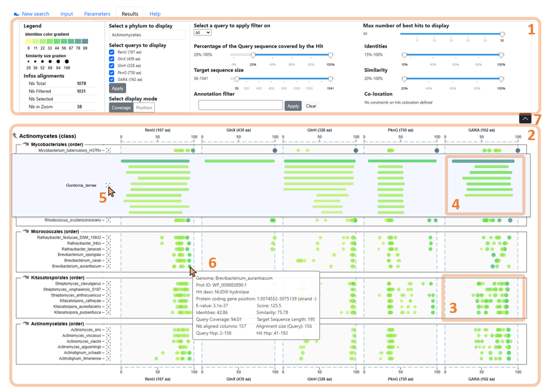 Figure 3: The WHOPPER browser with its key features for exploring alignment results.
The control panel (Figure 3.1) includes display options and real-time filtering features, and can be collapsed or expanded (Figure 3.7) to maximize results overview.
The hits chart (2) enables visualization of all alignments for query sequences (on the X-axis) against all proteomes (Y-axis), grouped by taxon. Hits can be displayed in two ways: (i) points representing their coverage (Figure 3.3) or (ii) bars showing their position (Figure 3.4).
The zoom feature (Figure 3.5) allows to display all the hits of a specific proteome. Hovering a hit displays its metadata (6).
Taxonomic navigation (Figure 4.8) allows the user to change the taxon and its sub-taxons displayed.
4. Select hits of interest
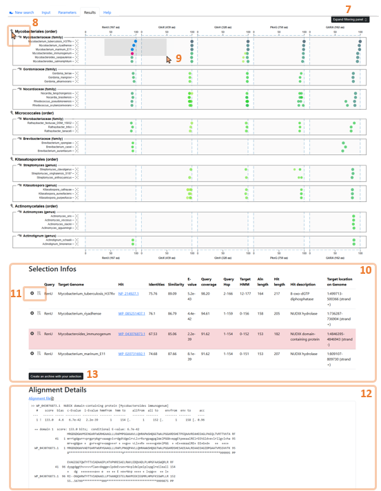 Figure 4: The WHOPPER browser with its key features on filtered alignments.
Hits are added to the selection directly on the graph by clicking on the hit to be added or by using a selection rectangle (Figure 4.9).
The combination (Ctrl + select) enables to add/remove new selection to current selection. Selected hits are shown in a table (Figure 4.10), located below the hits chart, associated with their metadata. From this table, hits can be highlighted or removed from the selection. The alignment details of the highlighted hit are displayed below the selection table (Figure 4.12). A hit can also be highlighted by double-clicking it on the chart.
5. Export selection
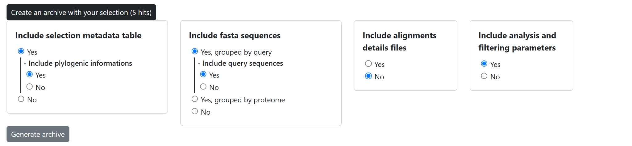 Figure 5: Export interface for downloading selected hits and associated metadata in WHOPPER.
The selection is available for download in different formats (Figure 5): fasta sequences grouped by query or genome, metadata with taxonomic information. The search parameters and the applied filters can also be downloaded.
Focus on: Genomic co-location filtering
1. Co-location constraint definition
When several query sequences have been used as input, it is possible to filter the results obtained on the basis of their genomic co-location.
A co-location constraint of the hits of query protein Q1 (called source) to the hits of a query protein Q2 (called target) is applied as follows:
For each hit of Q1, this one is retained if there is at least one hit of Q2 located at a maximum distance Dmax (cf Figure 8).
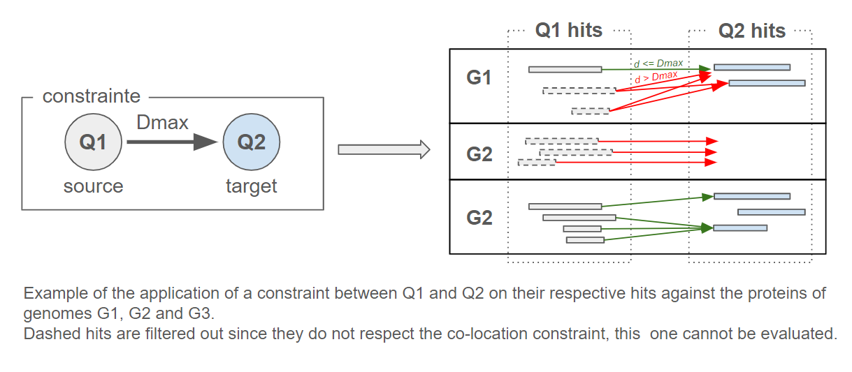 Figure 6: Illustration of co-location filtering. Hits of query Q1 are retained only if a Q2 hit is located within the specified maximum distance (Dmax) on the same genome.
The data used for this filter are the genomic coordinates of the protein-coding genes in each genome.
The distance d between two genes A and B is calculated as:
d = min(abs(start_B - stop_A), abs(start_A - stop_B))
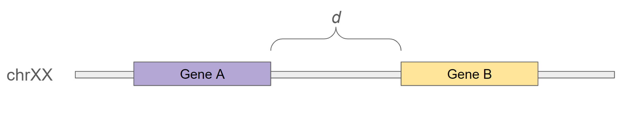 Figure 7: Genomic distance calculation between two genes. The distance
 d is defined as the minimal absolute gap between their start and stop positions.
It is possible to define severals co-location constraints to différents queries at the same time, with the following limitations :
- One query can be the “source” of only one constraint
- A query cannot have as its “target” a query for which it is itself a “target”.
Examples of allowed or not allowed constraints between query proteins :
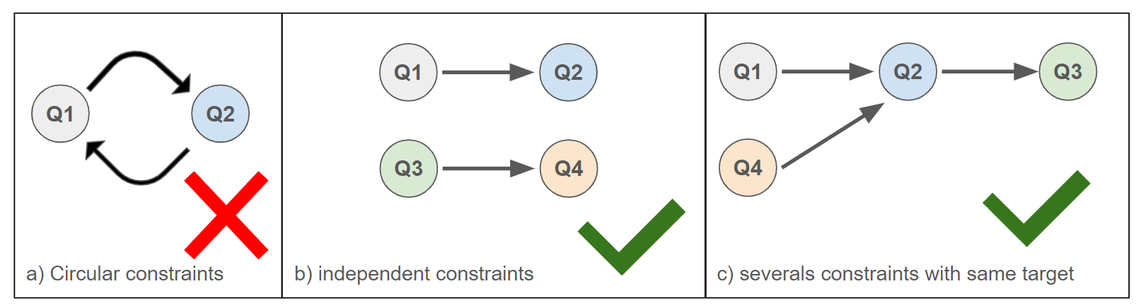 Figure 8: Examples of allowed and disallowed co-location constraints between query proteins.
Hits are always filtered from target hits to source hits. For example, in the case of figure 3.c, the successive filters are applied in the following order:
- filtering Q3 hits (coverage, identity, annotation, etc.)
- filtering of Q2 hits (coverage, identity, annotation, etc... ) + application of the Q2-Q3 co-location constraint on Q3 hits filtered in step 1.
- filtering of Q1 hits (coverage, identity, annotation, etc... ) + application of the Q1-Q2 co-location constraint to Q3 hits filtered in step 2.
- filtering of Q4 hits (coverage, identity, annotation, etc... ) + application of the Q4-Q2 co-location constraint to the Q2 hits filtered in step 2.
Note: using co-location constraints can slow down the application dramatically. It is therefore strongly recommended to perform a first filtering step on “target” queries which will serve as precise genomic anchors and limit the quantity of comparisons.
For example, in the case of figure 3.C it is recommended to filter accurately the Q3 hits before applying co-location constraints.
To apply a co-location constraint, first select the query sequence whose hits will be subject to the constraint by selecting it in the “Select query to apply filter on”
select box, then in the “Co-location constraint” section at the bottom right of the filter panel, in the select box to the right of the “nu max from” text field, select
the query whose hits will be used as starting points for the calculation. Finally, enter the maximum distance (in nucleotides) that must separate the hits of the two queries involved.
Notes:
- Co-location constraints only concern proteins in the same proteome.
- The distance between genes located on different chromosomes or scaffolds cannot be evaluated, in which case the co-location constraint is not satisfied. The level of completion and the quality of assembly for the different genomes used, as well as their level of annotation, are therefore critical factors that can have a significant impact on the results when using co-location constraints.
- Only one collocation constraint can be defined per query.
- By default, hits must be located on the same strand, but this constraint can be lifted by deactivating the “same strand required” option.
- Bidirectional/cyclic constraints such as A -> B & B -> A or A -> B & B-> & C -> A cannot be applied.
2. Use colocation constraints
When several query sequences have been used as input, it is possible to filter the results obtained on the basis of their genomic co-location.
To apply a co-location constraint, first select the query sequence whose hits will be subject to the constraint by selecting it in the
“Select query to apply filter on” select box, then in the “Co-location constraint” section at the bottom right of the filter panel, in the select
box to the right of the “nu max from” text field, select the query whose hits will be used as starting points for the calculation. Finally, enter
the maximum distance (in nucleotides) that must separate the hits of the two queries involved.
Example
The research focuses on identifying the homologs of proteins A, B and C, which are known to be present in the same operon. The genes encoding
these proteins therefore have genomic locations close to each other. By applying colocalization constraints, it is possible to identify all B and
C hits corresponding to proteins whose genes are located close to A hits.
To achieve this, the following filters are applied:
- Definition of a localization constraint between B and A hits:
- In the “Select query to apply filter on” select box, select value “B”.
- In the “Co-location constraint” text field, fill the value “10000”
- In the “Co-location constraint” select box, select the value “A”
- Definition of a location constraint between C and A hits:
- In the “Select query to apply filter on” select box, select value “C”
- In the “Co-location constraint” text field, fill the value “10000”
- In the “Co-location constraint” select box, select the value “A”
 Figure 9: Applying co-location constraints using the WHOPPER filter panel interface. The user selects the source query, defines the maximum distance, and chooses the target query.
Notes:
- In this example, only hits corresponding to proteins located 10,000 nucleotides upstream or downstream of A's hits on the same chromosome will be retained.
- In this example, A hits are used as a reference to filter out other hits. If no hits exist for A, all hits for B and C will be removed. It is therefore important to choose the right protein to use as a reference.